Mlsupervisedregression
Tabular Data - Concepts in Machine Learning - Supervisied Learning - Regression
Table of Content
Traditional Statistical Modeling vs Machine Learning
Traditional Statistical Modeling, we often know a good deal about the underlying process, thus we can choose a model of analysis that closely approximates that underlying process and use this to develop a predictive model.
Machine Learning on the other hand, we often know less about the underlying process or it’s too complicated to express, instead we learn or we approximate the equation from the data. Function approximation enables future values to be pridected using the machine learning model.
Machine Learning in Context with AI
Thinking Humanely -> Thinking Rationally | Acting Humanely -> Acting Rationally
The focus of machine learning will be honing in more on the “Thinking” processes (Thinking Humanly Thinking Rationally), and whether we’re trying to think specifically in regards to humanely or rationally will depend on our hope for the outcome.
Ex- With marketing we want to see how humans will react to certain comgaigns, whereas with supply chain optimization, we want to come up with the most rational means of producing and delivering products.
Thus Machine Learning will fall into the subset of AI define as when our machine is able to Learn.
Model: A Learning Algorithm
A model is a small thing that captures a larger thing, a good model is going to omit unimportant details while retaining what’s important.
Ex- World map, which represents a much larger reality.
In choosing the right representation or model, we always reduce the amount of information covered, but we need to do so in a way that preserves the features or relationships that we’re interested in.
A good model is able to do both; capture the important relationships and also reduce the complexity of a real world phenomenon enough for us to be able to take it in and understand and represents that real world.
Interpretation and Prediction:
Interpretation
We’re going to be training our model with the focus of finding insights about the data.
In the inerpretation approach, we look to our parameters to provide insight into our system. Generally, this will give us an idea of the different features that are providing the most value in predicting our outcome variable (target).
So our focus here is trying to understand the underlying difference in features that are going to affect our outcome variable (target).
The workflow will be gather x, y; train model by finding the parameters that gives the best prediction, but our main focus will be on the parameters themselves rather than the best prediction. So while we are indeed finding the best prediction, we may choose a less complex model to actually learn, so we’re optimizing for a specific model with high interpretability, rather than a model that may have high prediction power below interpretability since high interpretability is going to be our focus.
Examples |
|---|
Customer demographics vs sales data, where we care more about the loyalty by segments, in other words, what’s driving sales rather focusing on predicting what the future sales will be. |
Figure out the right safty features that will prevent accidents, so how can we adjust our safty features to prevent as many accidents as possible, rather than just trying to predict how many accidents a certain car will have, which would be important in its own right, but different in regards to our interpretation vs prediction trade-off. |
It could be the effect of our marketing budget on movie revenue, so we will know how much should we spend on our marketing budget, what does its effectiveness, rather than just trying to guess what a certain movie will actually have in box office revenue, which is again, is important in its own right. |
Predection
With the prediction approach, we’re focusing on how well our predictions will do compared to the actual values.
The focus here will be on performance metrics, this will just be some quantitatiev measure of the closeness between y_prediction and y, without focusing on interpretability, we risk having a black-box model, this will happen more often when we move to more complicated models like deep learning.
Examples |
|---|
We many not have the ability to control many features for customer churn, all we care about is correctly predicting the likelihood of a certain customer to churn. |
When predicting whether a certain customer will default, we will care much more about getting it right that getting the underlying interpretation (focus on predicting load defualt). |
Given past purchase history, what we can predict is just the future purchases, and that maybe more important that tying to figure out what the underlying factor is in regards to figure out those future purchases. |
For all these examples, we obviously would like to have interpretability of the underlying model, but if we think back to the interpretability examples, we obviously also wanted good prediction for those.
The idea is that there’s often going to be a trade-off, and when we’re using supervised machine learning for our own business example, we will have to think between choosing between a model that has high interpretability and a model that has high level of prediction, and that will have to be defined by your given business objective.
R2 metric:
:max_bytes(150000):strip_icc()/R-Squared-final-cc82c183ea7743538fdeed1986bd00c3.png)
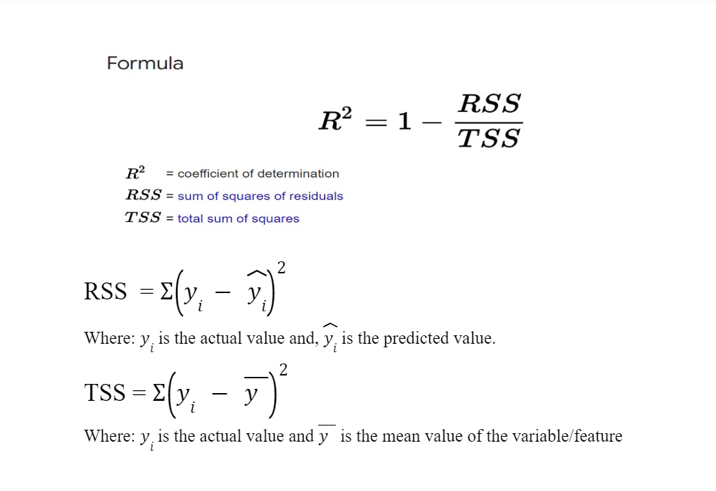
R2: Coefficient of Determination
The first component is going to be the sum squared error SSE, and that’s going to measure the distance between truth and our predictions.
The second part is going to be the total squared error TSS, which measures the distance between the truth and the average values of the truth.
So sum of squared error is the unexplained variation from our model, and the total squared error is the total variation.
So R2 is a measure of the explained variation by our model: 1 - (SSE/TSS), so we say how well our model explain the variation from the mean? How much was it able to reduce the amount of unexplained variance?
The Sum of Squared Errors (SSE) can be used to select the best-fitting regression model. Thus the closer this metric to 1 the better we did in regards to explaning the overall variance.
Note: keep in mind that as we make any model more complex, we can better fit to every single data point if we’d like, so we can always for example add on more features, and even if those features don’t have any predictive power, they will never bring down the R2 score. If you think about it if you were to add on another feature and it didn’t have any predictive power we could just set that coefficient to zero and it wouldn’t bring down our R2 because we will still be explaining the same amount of variation.
Features & Target Transformation
Making our target variable normally distributed often will lead to better results, but it is not necessary for linear regression for the target variable to be normally distributed, it may help and it’s worth trying, but it’s not necessary.
What is necessary for linear regression is that our errors are normally distributed. If our target is not normally distributed, we can apply a transformation to it and then fit our regression to predict the transformed values.
Notes:
For vanilla linear regression with no regularization, scaling actually doesn’t matter for performance.
If you’re taking a log transformation of some variables, you’re bring them down to a very similar scale as if you’re doing normal scaling.
Train-Test Split
Some transformations are done before we split the data into train and test like PloynomialFeatures which for example with degree= 2, will squares the features as well as interactions between each feature. Then we have something like StandardScaler which MUST be used after the train-test split, just keep in mind to apply it for both train and test.
When doing train-test splits make sure that your splits are independent from one another, often, parts of your test data can end up leaking into the training data, so that it’s not really unseen data, and we would actually learn to that test data. (Data Leakage)
One-Hot Encoding
When we do linear regrssion with one-hot encoding, for example; one-hot encoding if the location is beachfront or not .
1 |
0 |
5 |
0 |
1 |
4 |
As we can see here, the first column is corresponding to beachfront and the second not beachfront and the third is the price, if we don’t drop one of these columns, we can end up with an infine amount of different coefficients.
In order to define coefficient for the first column and second column, so imagine if we’r trying to get to the numbers 5 and 4 and start off with the intercept equal to 1 and then the coeeficient for our first column would be 4, so 1 + 4 = 5, but we also can start with the intercept being equal to 5 and the first coefficient equals to 0 thus 5 + 0 = 5, so if we don’t drop one of these columns (column one -beachfront- or column 2 -not beachfront-), we can end up with an infinite amount of what your INTERCEPT would be, because the first column and second column are completely dependent on one another; there is complete multicollinearity: when the first column is one the second column is always zero and vice versa. So let’s say we drop column 2 -not beachfront- [1, 5] [0, 4], then we can only have one option, for the second row our intercept will have to be 4, because we only have one coefficient which is -is is beachfront?- so for second row 4 + 0 = 4.
So that’s the danger of multicollinearity, it probabily won’t affect predictions, but it will affect the interpretability, but still best practice will generally be to drop one of these columns.
ohe= OneHotEncoder(drop= 'first')
One huge advantage of ohe over get_dummies is ohe returns a sparse matrix, which actually going to save alot of memory.

Cross Validation
A better way to validate our model is to use Cross Validation which going to calculate error across multiple train-test splits then we will average the resulting error for each one of these errors, it’s going to take more time, however, the performance measure is going to be more statistically significant.
Note that: the validation set must be mutually exclusive (independent and no overlap) from all of the other validation sets.
KFold
With KFold the training set can overlap but the test set have to be exclusive so that we are looking at different test sets every single time.
Pipeline; pipelines are going to allow you to chain together multiple operators on your data as long as they each have fit method, and then on top of that, every step leading up to the last step has to have a fit and transform so that the output of one can be the input of the next step, so you can chain together more than two steps as long as each one of those steps has fit_transform, and the last step has fit.
A high variance of parameter estimates across cross-validation subsamples indicates likely overfitting.
For a dataset with M observations and N features, Leave-one-out cross-validation is equivalent to k-fold cross-validation with k =M-1.
When using polynomial features and let’s say we get X and then X^2 which is a non-linear relationship between that feature and the target y, but the resulting algorithm is STILL LINEAR regression, since the outcome is still going to be a linear combination of the features that we have transformed into square of the original X variable that we are working with.
The non-linear relationship between one feature and the other is not going to make the algorithm non-linear as the algorithm itself still a linear combination of the different features that we have now created.
In K-fold cross-validation, how will increasing k affect the variance, increasing k will usually increase the variance of estimated parameters.
Bias-Variance Trade off:
Bias
Bias is a tendency to miss,
So for high bias and low variance: We are consistent, but we are consistently missing our target. That’s our tendency to miss.
Variance
Variance is tendency to be inconsistent
So for low bias and high variance: So low bias means you won’t have tendency to miss, but because high variance you be fairly inconsistent.
Idealy, we want to have low bias -less tendency to miss- and low variance -less tendency to be inconsistent-
We want to think about this tendency of our models as the expectation of out-of-sample behavior over many training set samples, so something like cross-validation would refer to our tendency to have high or low variance as well as high or low bias given our hold out sets. So that’s going to allow us to understand whether or not we have high bias, high variance, both high, or both low.
For Better Explanation of Bias-Variance, Please refer to chapter: fields/tabularData/dataEvaluation/modelBehaviour/biasVarianceTradeOff
Sources of Model Error
Source |
Explanation |
|---|---|
The model itself can be wrong (Bias) |
This will generally refer to models that are not doing well in identifying the relationship between our feature and target. This will generally be a bias model where our predictions are fairly consistent, but due to the model choice not properly defining the relationship between the X and y variable, we are consistently getting the wrong prediction. |
The model can be unstable (Variance) |
This generally relate to models with high variance, we can think our models are too perfectly identifying the relationship between X and y. So it’s actually incorporating random nosie besides the actual underlying function, and in that effort to perfectly define that relationship it may become unstable in their predictions. |
Unavoidable randomness (Irreducible Error) |
All our models are going to depend on real-world data, where there will always be a level of randomness within each one of our data points that we collect that could not be perfectly predicted. The idea is to find a model that finds the actual relationship while avoiding accidentally trying to incorporate this information that is just random noise. |
Bias |
Tendency of prediction to miss the true values, this can happen due to either missing infromation or overly simplistic models; think we are biased to the simplicity of our model or we are biased to the missrepresentation of our data given that missing data.High bias will happen when we missed the real pattern of our data, and we can associate high bias with the concept of underfitting or there not being enough complexity in our model. |
Variance |
Tendency of prediction is fluctuate, this is generally characterized by very high sensitivity of our output to small changes in our input.If you think about our overfit models that were too complex, we notice how a slight change in X values can end up with drastically different outcome y given the high fluctuation of our model. |
Model adjustments that decrease bias will often increase variance, and vice versa, we either biased to a very simple model or we can have high variance (high sensitivity) due to an overly complex model.
Regularization
The means by which our machine learns the parameters from the data is that we try minimize some cost function, for example minimizing the mean squared error for linear regression.
The new cost function with regularization will be that original cost function lets call it M(w), plus lambda multiplied by R(w), where R(w) is just going to be a function of the strength of our different parameters.
The regularization portion (lambda * R(w)) is added onto our original cost function so that we can penalize the model extra if it is too complex, essentially, this will allow us to dumb down the model, so the stronger our weights (the stronger our parameters), the higher this cost function (lambda * R(w)) is going to be, and we’re trying to ultimately minimize this, so we’re not going to be able to fit it as closely to the actual training data.
The lambda is going to add a penalty proportional to the size of the strenth of estimated model parameters, or it can be a function of these parameters, so the larger lambda is, the more we penalize stronger parameters, and again the more we penalize our model for being stronger and having stronger parameters, the less complex that model will be. That’ll make it so that we are trying to mizimize the strenth of all of our parameters while minimizing our original cost function.
Therefore, we’re going to increasing our original cost function according to how much we want to penalize our model for being more complex.
Regularization as Feature Selection
Regularization perform feature selection by shrinking the contribution of features since it’s going to take the contribution of each one of those features and eliminate or reduce them as it adds more weight to the penality.
So this is going to be most obvious with Lasso regression, for L1-reguralization this is accomplished by driving some of the coefficients in our linear regression down to zero.
It’s going to be the same effect as manual removing some features prior to modeling, except that with Lasso, it’ll find which ones to remove automatically according to some mathematical formula.
Another way to perform feature selection would be to just remove some of features right at the start, this would have to be done quantitatively, and a way that we can do this is remove a feature at a time and measure the predictive results via cross-validation, and if the feature elimination does improve the model on the holdout set or it doesn’t reduce the error that much, then we would say that we can probably safely remove that feature and perhaps even generalize better if that feature was not included.
Feature Selection
Why feature selection is improtant?
Reducing the number of features can prevent overfitting
For some models, fewer features can improve fitting time and/or results
Identifying most critical features can improve model interpretability
Keep in mind with original Linear Regression cost function, scaling would not have a large effect on our eventual outcome, but with Ridge Regression’s added coeffeicient weights to its cost function, scale will be of utmost importance, why?
let’s say X1 has value between 8 and 10, while X2 10000 and 20000 a 1 unit change will have a much larger coefficient in X1 compared to 1 unit change in X2, therefore if we end up with higher X1 coefficient we’ll end up being highly penalized for X1 coefficient.
Ridge Regression
Notes
The complexity penality lambda is going to be applied proportionally to the square of the coefficient values, so as we increase or decrease lambda what we’re doing is increasing or decreasing the effect of the square of each one of the coefficient values.
The penalty term has the effect of therfore “shrinking” our coefficients towards 0, not exacly 0 like Lasso, but the higher the coefficient is the more the penality is, therefore we want to be reducing the size of those coefficients.
This is going to impose bias on the model, but also reduce variance; the idea of regularization is inherently to reduce variance, which reduces the complexity of the model.
The penalty shrinks the magnitude of all of our coefficients by adding on the extra weight to our cost function, and larger coefficients are more strongly penalized because of the squaring // M(w) + [lambda * sum(w^2)] So a coefficient of 2 will be penalized x4 times as much as coefficient 1, because 1^2 = 1, and 2^2 = 4, so it will penalize larger weights even propotionally to the lower weight coefficients.
Value of Lambda |
Effect |
|---|---|
For a high lambda |
lambda value being high will be relative according to the coefficients that we have-, therefore we will end up with a high bias model -regularization was too much the model is now simple and cant fit well- because we put too much weight on the coefficients on our regularization term. |
For a middle value |
sweet spot- we have regularized our weights so it won’t be as complex as with no regularization, but also it won’t be as simple as the high lambda value |
For extreamly low value of lambda (even 0) |
we won’t have any regularization term. |
So as lambda increases the standardized coefficients should decrease so there should be inverse relationship, BUT we may see feature coefficient that can increase -temporary- while increasing lambda and other features are decreasing, and that would just be something due to multicollinearity, and at a certian point that feature will decrease as well, so all features decrease monotonically towards 0 once it reaches a certian threshold.
It’s possible that variance reduction may actually outpace the bias increase, so we can find a better fit model without having to increase bias too much, so what we mean is we can reduce the complexity while still consistently having enough information to show that relationship between X and y in our training set.
The idea here being that there may not necessarily be a linear trade-off between variance and bias, so we may be able to reduce complexity for some time while barely affecting the bias, and this may happen if we’re starting with an extreamly overfit model and we can keep reducing variance without increasing that bias.
Lasso Regression
Also Known for Least Absolute Shrinkage and Selection Operator
The main diiference between Lasso and Ridge is how we penalize the coefficients, with Ridge (L2), we use the coefficient squared, while with Lasso (L1) we’ll be using the absolute value of each one of these coefficients
Lasso is directly propotional to the absolute value of the coefficients, rather than with Ridge where it’s propotional to the square of the coefficients so don’t be askewed by the outliers.
Similar Ridge this will work by giving the user a mean to reduce complexity, an increase in lambda again will raise the bias and lower the variance and our complexity.
Lasso is more likely than Ridge to perform feature selection, meaning it’s more likely to completely zero out certain coefficients
The larger values of the coefficients are still going to be penalized, but again not as strongly as Ridge, with Ridge we squared the coefficients, so larger values had even more of a penality in relation to the coefficients.
The fact that it’s going to selectively shrink some coefficients compared to Ridge which is more likely to shrink all the coefficients at once. Lasso therefore actually eliminate certian features and perform feature selection for you, but it worth knowing that Lasso is slower to converge than Ridge due to the underlying optimization solution, so keep in mind the computation timing which will be faster for Ridge vs. perhaps higher interpretability of Lasso because once you remove certian features you can get a better idea of which features are actually improtant
Elastic Net
Elastic Net is an alternative hybird approach, introduces a new parameter alpha tht determines a weighted average of L1 (Lasso) and L2 (Ridge) penalities.
Recursive Feature Elimination (RFE)
It’s the tool that sklearn provides to do feature selection recursively and automatically, the way it works is:
First choosing the model; which model we want to limit the features of.
Second we explicitly define how many features we want to end up with.
Then RFE will repeatedly run the model, it will measure the different feature importances and recursively remove the less important features
The model that we choose to pass through must either have an attribute for the coefficients or for feature importance, and then the RFE will then eliminate the smallest value.
With that in mind we must ensure that we first scale our data if we’re going to do something like linear regression so that each one of the coefficients that are linear regression learns are going to be measured on the same scale.
Regularization under the hood
The Analytic View
The analytic view is going to present the obvious, as we incur L1 and L2 penalties, we force our coefficients to be smaller thus restricting their plausible range.
Think a smaller range for coefficients must imply a simpler model with lower variance than a model with an infinite possible coefficient range.
When we eliminate features (Lasso L1), this is clear, how we’re quickly eliminating that variance as we can just think of the difference between the possible solutions that are available for target y as a function of X only vs. being as function of X and X squared.
In regards to just shrinking coefficients (Ridge L2), so not necessarily eliminating coefficients we can think about how much that target y variable actually changes in response to a feature, so if the coefficient is close to 0, that’s essentially saying that, that feature has almost no effects, whereas if the coefficient is large, a small change in that feature will have a large impact on our target variable y, thus it will be higher sensitivity to a change in that feature and thus a higher vaiance in that underlying model.
Credits:
IBM Coursera Specialization